Focal spot position, collimator asymmetry¶

Now I will be using the Field size module of QAserver.

As I have demonstrated in the Winston-Lutz section, it is possible to detect with the WL test whether the focal spot of the beam is not on the collimator axis of rotation. Measurements with two sets of images are needed: one with collimator angles 0/180, and another with collimator angles 90/270. In both cases the field must be shaped both with diaphragms and MLCs. If the measured longitudinal shifts of the BB differ, there is a GT deviation of the focal spot. A potential AB deviation can be seen from a single acquisition.

6 MV focal spot position and adjustment¶

Please read these two articles:

Nyiri BJ, Smale JR, Gerig LH, Two self-referencing methods for the measurement of beam spot position, Med Phys. 2012 Dec; 39(12):7635-43 (https://www.ncbi.nlm.nih.gov/pubmed/23231311)
Chojnowski JM, Taylor LM, Sykes JR, Thwaites DI, Beam focal spot position determination for an Elekta linac with the Agility® head; practical guide with a ready-to-go procedure, J Appl Clin Med Phys. 2018 Jul;19(4):44-47 (https://www.ncbi.nlm.nih.gov/pubmed/29761625/)

So, basically, if the focal spot is not on the collimator axis of rotation, you will get a wobbling CAX when the collimator is rotated. But not because of MLC or diaphragm asymmetry, but because diaphragms and MLCs are at different levels along the beam line.

I always focus on 6 MV. This is the reference beam. All other beams should be aligned to it. The hardest thing to detect and adjust is the GT deviation. If you miss by 0.1-0.3 mm at the isocenter, no matter. In the clinical setting you can compensate this with XVI’s flexmaps, so that at the end of the day you will not be missing small tumors.

Here is my measurement process with QAserver:

Set the optical crosshair to align with the collimator axis of rotation.
Put Elekta’s Agility calibration plate on the couch and align it with the crosshair.
Image the plate with a large field. Then with a field size of 7 cm x 7 cm acquire four images at collimator angles 270, 0, 90 and 180. Make sure the field is shaped with diaphragms and MLCs.
Analyze the images.

1. Setting the optical crosshair¶

Put a piece of paper on the couch, make a very very very small mark on the paper. Align the mark with the optical crosshair center. Rotate the collimator. There should be absolutely no wobble of the optical crosshair when the collimator is rotated. If there is even a small amount of wobble that is not caused by collimator eccentricity, have the crosshair adjusted.

If you wish to measure the true deviation of the radiation field from the light field, you can place a metal marker on the epid. But, in this case the optical crosshair must be very accurate 60 cm under the isocenter.

2. Setting Elekta’s Agility plate¶

Set gantry and collimator angles to 0. Put on the couch Elekta’s Agility calibration plate at SSD = 100 cm. Align the plate with the crosshair.

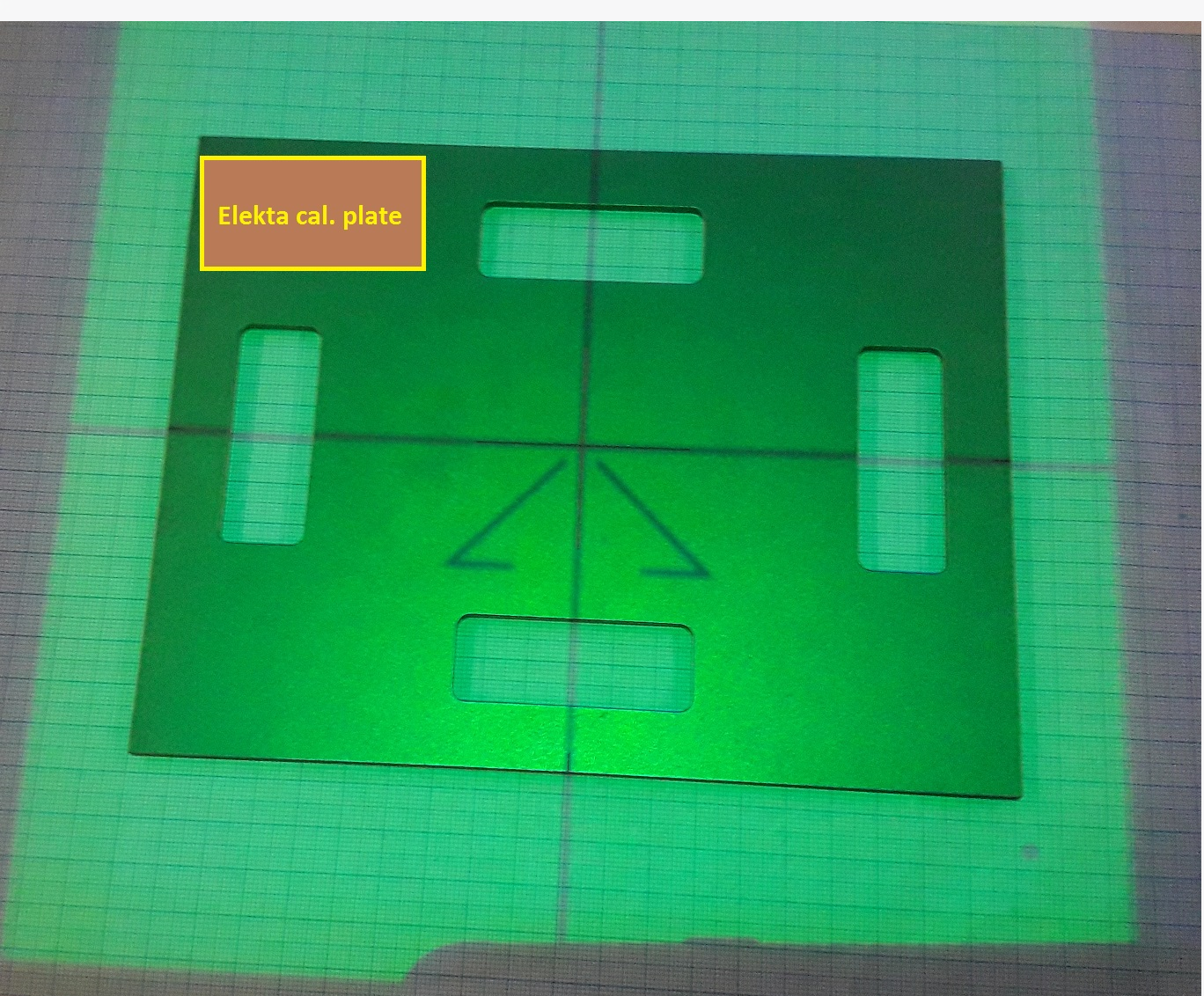
Elekta’s calibration plate accurately aligned with the crosshair.¶

3. Acquiring images¶

Create a treatment in iView. Create a new Field. Make an EPID image of the plate first. Use a field size of 24 cm x 24 cm. Use at least 20 MU. Make sure you don’t have the edge of the couch in the image.

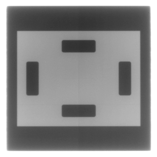
Image of Elekta’s plate.¶

While the plate is still on the couch, acquire four images of a square field 7 cm x 7 cm shaped with diaphragms and MLCs at collimator angles 270, 0, 90 and 180. Use at least 20 MUs. If you want, you can remove the plate and use larger fields, just don’t move the gantry, or the EPID!

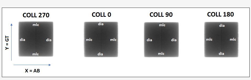
An image of a 7 x 7 field. The field goes through the metal plate.¶

Repeat this many, many times. One single measurement will not suffice.

4. Analyzing images¶

In article 2 you can read how to extract focal spot deviation from the measurements. The Field size module gives you the position of the field CAX at the isocenter with respect to the center of the plate (mechanical marker). We will use these measurements to calculate focal spot deviation. Image below shows Agility head geometry. A marker is positioned onto the collimator axis of rotation. Note that the deviating beam projects the marker on the epid away from the collimator axis of rotation. So if you would like to measure the true beam deviation from the collimator axis of rotation, you should put the marker on the epid.

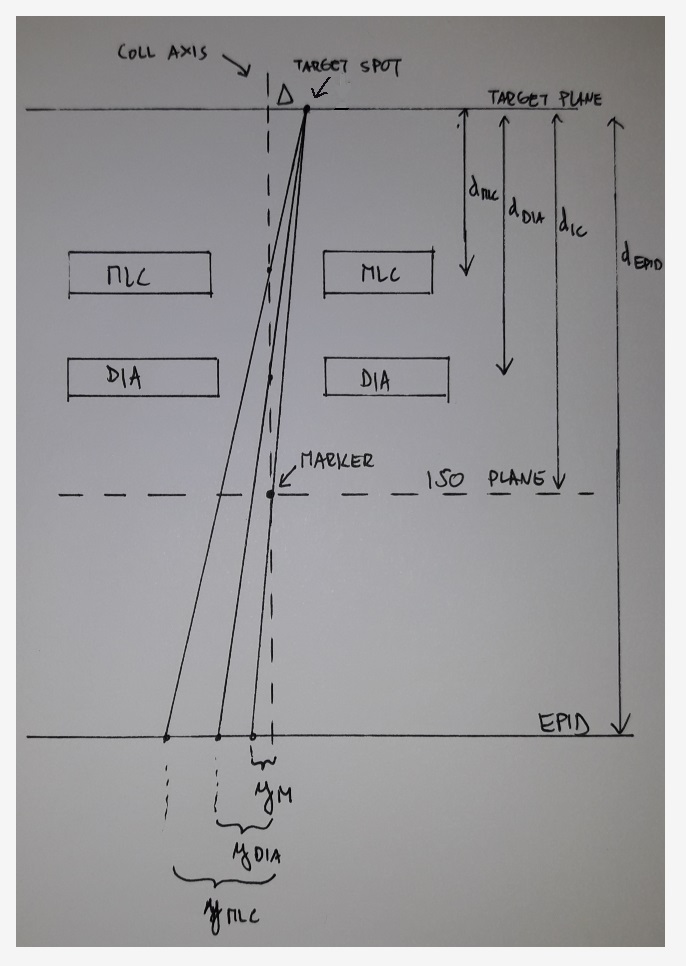
Agility head geometry (see article 2).¶

Two pairs of similar triangles give:

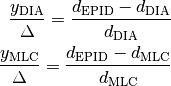
$\frac{y_\mathrm{DIA}}{\Delta} = \frac{d_\mathrm{EPID}-d_\mathrm{DIA}}{d_\mathrm{DIA}}\\ \frac{y_\mathrm{MLC}}{\Delta} = \frac{d_\mathrm{EPID}-d_\mathrm{MLC}}{d_\mathrm{MLC}}$

Where

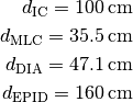
$d_\mathrm{IC}=100 \,\mathrm{cm}\\ d_\mathrm{MLC}=35.5 \,\mathrm{cm}\\ d_\mathrm{DIA}=47.1 \,\mathrm{cm}\\ d_\mathrm{EPID}=160 \,\mathrm{cm}$

If we had the measurements at the EPID plane, the focal spot deviation would be

$\Delta = \frac{y_\mathrm{MLC}-y_\mathrm{DIA}}{d_\mathrm{EPID} \left(\frac{1}{d_\mathrm{MLC}} - \frac{1}{d_\mathrm{DIA}}\right)} = 0.908\left(y_\mathrm{MLC}-y_\mathrm{DIA}\right)$

But the Field size module will give you field CAX deviation at the isocentric plane (marker plane). Therefore, we must project the results to the isocentric plane. At the isocentric plane we denote the deviations with an apostrophe.

$\Delta = \frac{y'_\mathrm{MLC}-y'_\mathrm{DIA}}{d_\mathrm{IC} \left(\frac{1}{d_\mathrm{MLC}} - \frac{1}{d_\mathrm{DIA}}\right)} = 1.453\left(y'_\mathrm{MLC}-y'_\mathrm{DIA}\right)$

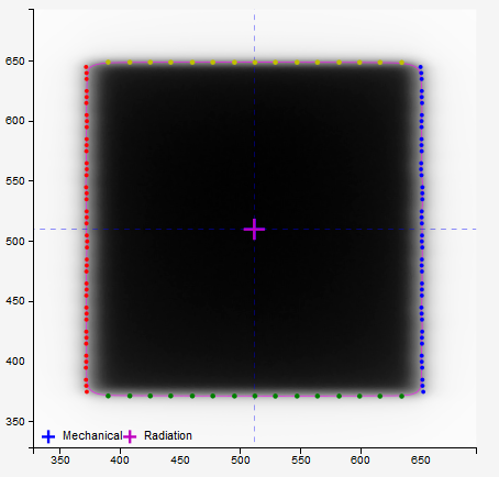
So this is the focal spot deviation. Collecting $y'_\mathrm{MLC}$ and $y'_\mathrm{DIA}$ goes like this. Send the images to QAserver. Open the Field size module. Set the first image to the image of the plate, and for “set center” choose Plate. The second image should be one of the 7 x 7 field images. Run the analysis. For each 7 x 7 image collect the “Radiation center offset from mechanical center” results, denoted as $\Delta X$ and $\Delta Y$ .

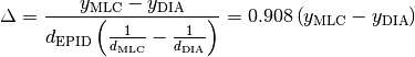
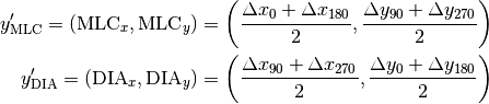
Calculate the center of the MLC shaped field and the center of the diaphragm shaped field (at isocentric plane):

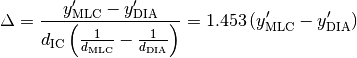
$y'_\mathrm{MLC} = \left(\mathrm{MLC}_x, \mathrm{MLC}_y\right)=\left(\frac{\Delta x_0+\Delta x_{180}}{2}, \frac{\Delta y_{90}+\Delta y_{270}}{2} \right)\\ y'_\mathrm{DIA} = \left(\mathrm{DIA}_x, \mathrm{DIA}_y\right)=\left(\frac{\Delta x_{90}+\Delta x_{270}}{2}, \frac{\Delta y_{0}+\Delta y_{180}}{2} \right)$

Now, the average deviation of the beam, taking both MLC and DIA shaped fields into account, at the isocentric plane is approximately:

$\textrm{Iso. dev.} = \frac{y'_\mathrm{MLC}+y'_\mathrm{DIA}}{2} = \frac{\Delta}{2}\left(\frac{d_\mathrm{IC}}{d_\mathrm{DIA}}+\frac{d_\mathrm{IC}}{d_\mathrm{MLC}}-2\right) = 1.47\Delta$

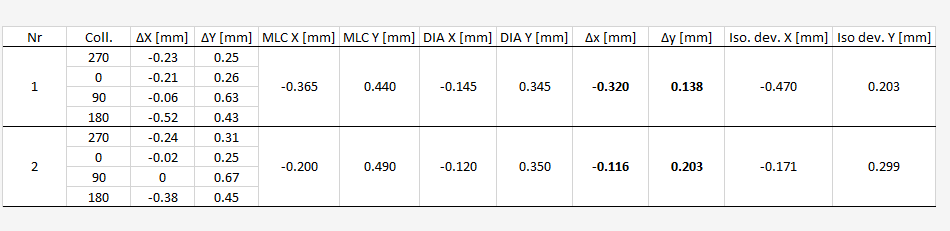
Two measurements for 6 MV.¶

The table shows two measurements of focal spot position done in sequence. Because of some problems with MLC positioning that I had, the measurements differ significantly. Many more repetition of this measurement are necessary to get a reliable results in any case.

Warning

Doing one single measurement or two is not enough to definitively tell whether the focal spot is not on the collimator axis of rotation. It is also prudent to establish the same result with the WL test before any adjustments are planned.

If the focal spot position deviation, when projected to the isocenter, deviates too much, it will not be possible to calibrate Agility. I like to measure this frequently just to see what is going on with the beam. Normally, there is no significant change over time. But if the Agility calibration workflow warns of a larger deviation, and if it is confirmed by your measurements, then your service engineers could use your data to more confidently adjust beam steering, if needed.

Note

Before you collect measurements of the focal spot position that you would like to show to your service engineers, make sure the beam is optimized, especially Gun I and 2T/2R.

5. The effect of Bending fine on focal spot position¶

In the above case it turned out, when I repeated the measurements over several months, and analyzed the WL results as well, that the largest deviation was in the GT direction. The magnitude of this deviation was rounded to 0.3 mm. This can be remedied with Bending fine adjustment. Bending fine moves the beam in the GT direction without introducing a significant tilt to the beam. Compare the above table with the following one. Both tables contain measurement performed with the same plate position in the time spacing of several minutes (just for demonstration). Bending fine was increased by 100 mA between the pairs of measurements.

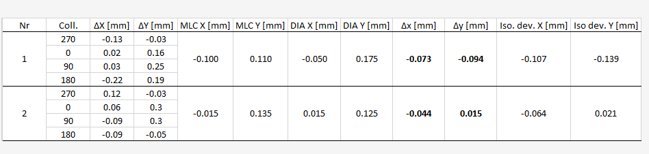
Two measurements for 6 MV. Both with increased Bending fine (100 mA). The plate is in the same position as for the measurements in the previous table. Note how the deviations came down.¶

A 100 mA increase in Bending fine pushes the beam by about 0.2-0.3 mm towards T. In this test, 2R/2T were not adjusted for better symmetry after the change in Bending fine. I leave it to experienced engineers to set everything correctly.

Multiple radiation isocenters¶

Each energy has its own “isocenter”, that is to say, each energy has an independent focal spot position. One should therefore do the same test for other energies. For example, for 6 MV, 10 MV and 15 MV, on a good day I would get this:

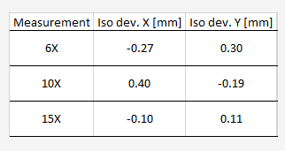
Isocenter deviations for 6 MV, 10 MV and 15 MV. The reference is the collimator axis of rotation (optical crosshair).¶

The above results clearly show that 10 MV does not align well with 6 MV. What is the consequence of this? Luckily, 6 MV has no significant lateral deviation. This means that a good flexmap calibration will teach XVI to position the tumor into the center of this beam, which is displaced by 0.24 mm towards G. Treating with this beam will be accurate. But, with the 10 MV beam we will miss the tumor by 0.5 mm longitudinally. Three options remain. One, leave it like it is. Two, push 10 MV closer to 6 MV. Three, fix all beams to be closer to 6 MV, and make 6 MV closer to the collimator axis of rotation. In such a situation I would probably choose option 2.

Asymmetry and Agility workflows¶

My summary of what to watch for when engineers calibrate Agility would be this:

Make sure that the optical crosshair is always accurate.
If the optical system is removed or even slightly disturbed, you will notice a difference in leaf positioning. A STW (Setting To Work) re-calibration should be done always. It will save you time with double testing if you just do it right after maintenance.
Before calibration do tests of the optical field. Change field sizes and observe how MLC leaves and diaphragms move to final position. If you notice that the whole leaf bank is moving about, trying to find a fixed position, then you have a problem that will affect the calibration process.
Do regular tests of focal spot position. Average measurements over several days. The measurements should be stable. If you have a larger deviation, in my experience more than 0.3 mm, you will have problems with Agility calibration.
Do not disregard Leaf bank height and lateral setup! Particularly if the whole BLD (Beam Limiting Device) was removed for maintenance and then put back on. A bad setup will cause MLC/diaphragm asymmetry.

Warning

Do not run workflows yourself, you may cause a miss-calibration.

Collimator asymmetry¶

You can measure this with the Winston-Lutz module, or with the Field size module. Acquire two images of a field, say 7 x 7, at two opposite collimator angles 0/180. Measure the spacing between the centers of the fields. This is quickly achieved in the Field size module by setting the first image as Image 1 and the opposite coll angle image as Image 2, and using the “CAX” method for Set center. This will give you an estimate of the asymmetry of MLC/diaphragm positioning. I usually measure at collimator angle pairs 90/270 as well. The table below demonstrates 10 measurements in one session. MLC leaves have a small average asymmetry of about 0.5 mm. Diaphragms do not have a significant asymmetry.

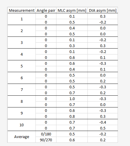
Measurements of MLC and diaphragm asymmetry with a field size of 7 x 7. The asymmetry in this table is presented as the distance between field centers at opposite collimator angles.¶

When this asymmetry (difference between centers) reaches 0.4 mm, you should report it to your service engineers. They should re-calibrate Agility, and also run the Leaf bank height and lateral setup workflow. Agility normally has asymmetry of about 0.2 mm. It is a fantastic collimator!

Now, as a physicist I should complicate this a bit. To get a real grasp of what is wrong with the collimator, what is the error in positioning of each leaf bank and each diaphragm, one should do a more sophisticated measurement. If, for example, you rotate the collimator, and you get a 0.4 mm displacement between the centers, this does not mean that one bank is off by 0.2 mm, and the other by the same 0.2 mm. It could be 0.1 mm and 0.5 mm, or 0.1 mm and 0.3 mm. It depends on the direction of the error.